1. Review of Linear Equations and Inequalities
A linear equation of two variables xxx and yyy is of the form:
ax+by+c=0ax + by + c = 0ax+by+c=0
A linear inequality in two variables (x and y) is an expression of the form:
ax + by + c > 0
ax + by + c < 0
ax + by + c ≥ 0
ax + by + c ≤ 0
Where:
a, b, c are constants (numbers)
x, y are variables
Example: x≥3x \ge 3x≥3
Number of variables: 1 (xxx)
Sign ≥\ge≥ means all values of xxx greater than or equal to 3
Boundary line: The equation x=3x = 3x=3 is a straight line parallel to the y-axis. It divides the plane into two parts:
Right of line: x>3x > 3x>3
Left of line: x<3x < 3x<3
Points on the line: x=3x = 3x=3
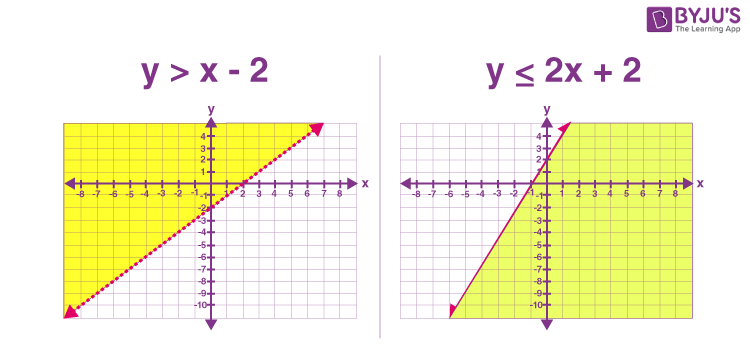
Solid line: used if the inequality includes equality (≥\ge≥ or ≤\le≤)
Dotted line: used if strict inequality (>>> or <<<)
2. Graph of Inequalities in Two Variables
Example: 2x+3y≥62x + 3y \ge 62x+3y≥6
Corresponding equation (boundary line): 2x+3y=62x + 3y = 62x+3y=6
Make a table of points:
x 0 3 6
y 2 0 -2
Plot the points (0,2), (3,0), (6,-2) and join with a solid line
Test a point (e.g., origin (0,0)) in the inequality:
2(0)+3(0)≥6 ⟹ 0≥6 (False)2(0) + 3(0) \ge 6 \implies 0 \ge 6 \text{ (False)}2(0)+3(0)≥6⟹0≥6 (False)
Hence, the feasible region does not contain the origin; shade the opposite side.
Example: 2x−3y<62x - 3y < 62x−3y<6
Boundary line: 2x−3y=62x - 3y = 62x−3y=6
Table of points:
x30-3y0-2-4
Join points with dotted line (since < does not include equality)
Test point (0,0): 0−0<60 - 0 < 60−0<6 → True → shade region containing origin
Note: If boundary line passes through origin, choose a different test point (1,0) or (0,1).
3. System of Linear Inequalities
A system of linear inequalities consists of two or more inequalities with a common solution region.
Example: x−2y≥4x - 2y \ge 4x−2y≥4 and 2x+y≤82x + y \le 82x+y≤8
Boundary lines:
x−2y=4x - 2y = 4x−2y=4
2x+y=82x + y = 82x+y=8
Make tables and plot points for each line
Test the origin (0,0) in each inequality to identify which region to shade
The intersection of shaded regions is the solution set
4. Linear Programming (L.P)
Definition: A mathematical technique to maximize or minimize an objective function under given constraints.
Basic Terms
Decision variables: Variables whose values are to be determined (e.g., x,yx, yx,y)
Objective function: Linear function to be optimized (e.g., F=4x−yF = 4x - yF=4x−y)
Constraints: Conditions the decision variables must satisfy (e.g., 2x+3y≥62x + 3y \ge 62x+3y≥6)
Feasible region: Closed area on the graph where all constraints overlap
Feasible solution: Any point in the feasible region satisfying all constraints
Maximum/Minimum values: Always occur at the vertices of the feasible region
5. Steps to Solve L.P Problems
Identify decision variables and objective function
Convert constraints into equations (boundary lines)
Plot boundary lines on a graph
Solid line if ≤\le≤ or ≥\ge≥
Dotted line if < or >
Identify feasible region (intersection of all constraints)
Find vertices of feasible region
Evaluate objective function at each vertex
Select maximum and minimum values
6. Example Problems
Example 1: Maximize/Minimize F=4x−yF = 4x - yF=4x−y
Constraints: 2x+3y≥62x + 3y \ge 62x+3y≥6, 2x−3y≤62x - 3y \le 62x−3y≤6, y≤2y \le 2y≤2
Boundary lines:
2x+3y=62x + 3y = 62x+3y=6 → points (0,2),(3,0),(6,-2)
2x−3y=62x - 3y = 62x−3y=6 → points (3,0),(0,-2),(-3,-4)
y=2y = 2y=2 → horizontal line
Feasible region: ΔABC\Delta ABCΔABC with vertices A(3,0), B(6,2), C(0,2)
Evaluate F=4x−yF = 4x - yF=4x−y at vertices:
A: 12
B: 22 (Max)
C: -2 (Min)
Example 2: Max/Min Z=2x+yZ = 2x + yZ=2x+y
Constraints: x+y≤6x + y \le 6x+y≤6, x−y≤4x - y \le 4x−y≤4, x≥0x \ge 0x≥0, y≥0y \ge 0y≥0
Boundary lines:
x+y=6x + y = 6x+y=6 → points (0,6),(6,0)
x−y=4x - y = 4x−y=4 → points (0,-4),(4,0)
x=0x = 0x=0, y=0y = 0y=0
Feasible region: quadrilateral OABC with vertices O(0,0), A(4,0), B(5,1), C(0,6)
Evaluate Z=2x+yZ = 2x + yZ=2x+y:
O: 0 (Min)
B: 11 (Max)
Example 3: Given ∆ABC with vertices A(2,0), B(6,0), C(1,4) and objective function F=2x+3yF = 2x + 3yF=2x+3y
Boundary inequalities:
BC: 4x+5y≤244x + 5y \le 244x+5y≤24
AC: 4x+y≥84x + y \ge 84x+y≥8
AB: y > 0, x > 0 (first quadrant)
Minimum value of FFF occurs at A: F=4F = 4F=4
Example 4: Maximize P = 3x + 2y
Constraints:
x + y ≤ 6
x ≤ 4
y ≤ 3
x ≥ 0, y ≥ 0
Steps:
Draw boundary lines:
x + y = 6 → points (0,6) or (6,0)
x = 4 → vertical line through x = 4
y = 3 → horizontal line through y = 3
Feasible region: Quadrilateral with vertices A(0,0), B(4,0), C(4,2), D(3,3)
Evaluate P = 3x + 2y at vertices:
A: 0 or B: 12 or C: 16 (Max) or D: 15
Answer: Max P = 16 at (4,2), Min P = 0 at (0,0)
Example 5: Minimize Z = 5x + 4y
Constraints:
2x + y ≥ 4
x + 2y ≥ 6
x ≥ 0, y ≥ 0
Steps:
Draw boundary lines:
2x + y = 4 → points (0,4) or (2,0)
x + 2y = 6 → points (0,3) or (6,0)
Feasible region: Triangle with vertices A(2,0), B(0,3), C(4/3, 4/3)
Evaluate Z = 5x + 4y at vertices:
A: 10 or B: 12 or C: 20/3 + 16/3 = 12
Answer: Min Z = 10 at (2,0)
Example 6: Maximize F = x + y
Constraints:
x + 2y ≤ 8
3x + y ≤ 9
x ≥ 0, y ≥ 0
Steps:
Boundary lines:
x + 2y = 8 → points (0,4) or (8,0)
3x + y = 9 → points (0,9) or (3,0)
Feasible region: Quadrilateral with vertices A(0,0), B(0,4), C(2,3), D(3,0)
Evaluate F = x + y at vertices:
A: 0 or B: 4 or C: 5 (Max) or D: 3
Answer: Max F = 5 at (2,3), Min F = 0 at (0,0)
Example 7: Maximize Profit P = 7x + 5y
Constraints:
x + y ≤ 10
x ≤ 6
y ≤ 8
x ≥ 0, y ≥ 0
Steps:
Boundary lines:
x + y = 10 → points (0,10) or (10,0)
x = 6 → vertical line
y = 8 → horizontal line
Feasible region: Quadrilateral with vertices A(0,0), B(6,0), C(6,4), D(2,8)
Evaluate P = 7x + 5y at vertices:
A: 0 or B: 42 or C: 76+54=42+20=62 (Max) or D: 14+40=54
Answer: Max P = 62 at (6,4), Min P = 0 at (0,0)
Example 8: Minimize C = 2x + 3y
Constraints:
x + y ≥ 5
2x + 3y ≥ 12
x ≥ 0, y ≥ 0
Steps:
Boundary lines:
x + y = 5 → points (0,5) or (5,0)
2x + 3y = 12 → points (0,4) or (6,0)
Feasible region: Triangle with vertices A(0,5), B(6,0), C(3,2)
Evaluate C = 2x + 3y at vertices:
A: 20+35=15
B: 26+30=12 (Min)
C: 23+32=6+6=12
Answer: Min C = 12 at (6,0) or (3,2), Max C = 15 at (0,5)
7. Important Notes
The feasible region is always convex
Maximum/minimum values always occur at vertices
Always test a point to determine which side of the boundary line to shade
Solid line includes the line, dotted line excludes the line
Visit this link for further practice!!
https://besidedegree.com/exam/s/academic